The `` sliding motion'' described above suggests a way for identifying
the optimal values for, let's say, a max LP problem. The underlying
idea is to keep ``sliding'' the isoprofit line ![]() in the direction of increasing
in the direction of increasing ![]() 's, until we cross
the boundary of the LP feasible region. The implementation of this
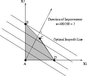
idea on the prototype LP of Equation 5 is depicted in
Figure 3.
's, until we cross
the boundary of the LP feasible region. The implementation of this
idea on the prototype LP of Equation 5 is depicted in
Figure 3.

Figure 3: Graphical solution of the prototype example LP
From this figure, it follows that the optimal daily production levels
for the protoype LP are given by the coordinates of the point
corresponding to the intersection of line ![]() with the
with the ![]() -axis, i.e.,
-axis, i.e., ![]() . The maximal daily profit is
. The maximal daily profit is ![]() . Notice that the optimal point is one of
the ``corner'' points of the feasible region depicted in
Figure 3. Can you argue that for the geometry of the
feasible region for 2-var LP's described above, if there is a bounded
optimal solution, then there will be one which corresponds to one of
the corner points? (This argument is developed for the broader context
of n-var LP's in the next section.)
. Notice that the optimal point is one of
the ``corner'' points of the feasible region depicted in
Figure 3. Can you argue that for the geometry of the
feasible region for 2-var LP's described above, if there is a bounded
optimal solution, then there will be one which corresponds to one of
the corner points? (This argument is developed for the broader context
of n-var LP's in the next section.)