Consider the constraint:
The solution space of this constraint is one of the closed
half-planes defined by the equation: ![]() . To show
this, let us consider a point
. To show
this, let us consider a point ![]() which satsifies
Equation 10 as equality, and another point
which satsifies
Equation 10 as equality, and another point
![]() for which Equation 10 is also valid. For
any such pair of points, it holds that:
for which Equation 10 is also valid. For
any such pair of points, it holds that:
Interpreting the left side of Eq. 11 as the inner
(dot) product of the two vectors ![]() and
and ![]() , and recognizing that
, and recognizing that ![]() , it follows that line
, it follows that line ![]() ,
itself, can be defined by point
,
itself, can be defined by point ![]() and the set of points
and the set of points
![]() such that vector
such that vector ![]() is at right angles
with vector
is at right angles
with vector ![]() . Furthermore, the set of points
. Furthermore, the set of points ![]() that satisfy the > (<) part of Equation 11 have the
vector
that satisfy the > (<) part of Equation 11 have the
vector ![]() forming an acute (obtuse) angle with vector
forming an acute (obtuse) angle with vector
![]() , and therefore, they are ``above'' (``below'') the line.
Hence, the set of points satisfying each of the two inequalities
implied by Equation 10 is given by one of the two
half-planes the boundary of which is defined by the corresponding
equality constraint. Figure 1 summarizes the above
discussion.
, and therefore, they are ``above'' (``below'') the line.
Hence, the set of points satisfying each of the two inequalities
implied by Equation 10 is given by one of the two
half-planes the boundary of which is defined by the corresponding
equality constraint. Figure 1 summarizes the above
discussion.
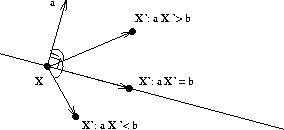
Figure 1: Half-planes: the feasible region of a linear inequality
An easy way to determine the half-plane depicting the solution space of a linear inequality, is to draw the line depicting the solution space of the corresponding equality constraint, and then test whether the point (0,0) satisfies the inequality. In case of a positive answer, the solution space is the half-space containing the origin, otherwise, it is the other one.
From the above discussion, it follows that the feasible region for the prototype LP of Equation 5 is the shaded area in the following figure:
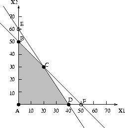
Figure 2: The feasible region of the prototype example LP