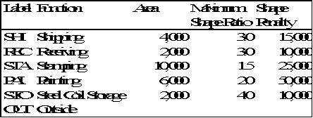


The company produces stamped metal parts, to be used in automotive assembly, from sheetmetal coils. The plant consists of five major departments. Some of the parts have to be treated with corrosion resistive paint and then dried in an oven. Forklift trucks are used for all material handling transportation operations in the plant. A summary of the department data is given in Table 4.5. The number of truck trips per week between each pair of departments and between each department and the outside is given in Table 4.6. The building dimensions are 200 by 120 feet.
Table 4.5. Department Data for the Autoparts Example

Table 4.6. Material Handling Trips for the Autoparts Example
We will first create a hexagonal adjacency graph and block layout following the SPIRAL methodology. For the graph construction phase, we will use the binary relationships, not use improvement interchanges, and break location ties by the centroid-seeking rule. For the graph, we will show first the symmetrical adjusted relationships in a two-dimensional matrix. We then will show the sorted list of adjusted binary relationships. Third, we will show the adjacency graphs after we have added each department. Finally, we will compute and show the adjacency and efficiency score of the final graph.
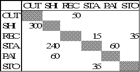
We first convert the asymmetrix material handling trips to a symmetric relationship table, where all relationships are shown above the main diagonal.
Table 4.7. Symmetric Relationships for theAutoparts Example
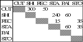
Next the adjusted binary relationships, that incorporate the relationships with the outside, are computed. Because several departments have positive relationships with the outside, many of the adjusted relationships are negative.
Table 4.8. Binary Adjusted Relationships for the Autoparts Example
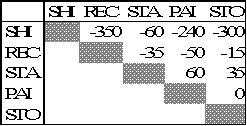
The adjusted binary relationships are then sorted in decreasing order.
Table 4.9. Sorted Binary Adjusted Relationships for the Autoparts Example

The first two departments to enter the hexagonal adjacency graph are the two departments in the first element of the list, i.e. STA and PAI. They are placed at random in two adjacent vertices of the hexagonal grid.
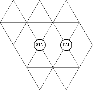
Figure 4.15. Adjacency Graph with 2 Departments for the Parts Example
The next relationship selected must have one department in the graph and one department not in the graph. These departments are called the anchor department and the new department, respectively. The anchor department also must have an open adjacent grid position. Element two of the list satisfies all those conditions: department STA is in the graph, department STO is not, and department STA has an empty adjacent grid position. All empty grid positions adjacent to the anchor department are possible locations for the new department, and because of the relationship selection rule there exists at least one open adjacent grid position. The grid position with the highest adjacency score based on the original symmetric relationships is selected. Ties are broken by the centroid-seeking rule, i.e. the new department is located in the open grid location adjacent to the anchor department that tied for the highest adjacency score and that is closest to the centroid of the current adjacency graph. Department STO has only a relationship with department STA, and thus all open grid positions adjacent to department STA are tied. There are three grid position closest to the centroid of the graph and the one above the centroid is selected at random.
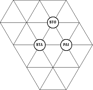
Figure 4.16. Adjacency Graph with 3 Departments for the Autoparts Example
Element four is the next relationship selected from the list. Department STO is in the graph, department REC is not, and department STO has an open adjacent grid position. Deparment REC has a positive relationship with departments STA and STO and so the open grid position adjacent to both those department is the selected location for department REC.
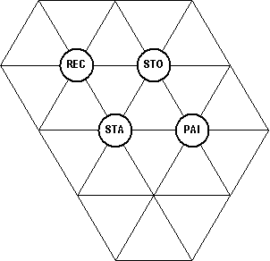
Figure 4.17. Adjacency Graph with 4 Departments for the Parts Example
Department SHI is the only remaining free department. Element seven is the next selected relationship, since department STA is in the graph, deparment SHI is not in the graph, and department STA has an open adjacent grid location. All open grid positions adjacent to department STA are candidate locations. Since department SHI has positive relationships only with departments STA and PAI, it will be located in the open grid location adjacent to those two departments.
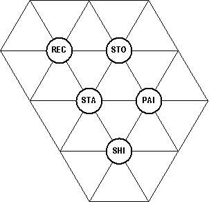
Figure 4.18. Adjacency Graph with 5 Departments for the Parts Example
To compute the adjacency score, we construct the adjacency matrix for the graph above.
Table 4.10. Adjacency Matrix for the Autoparts Example
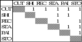
The adjacency matrix is then multiplied element by element with the symmetrical relationship matrix and the sum of the product is computed. The sum is equal to 795. Since the sum of the absolute values of all relationships is also equal to 795, the efficiency of the above graph is equal to 100 %.
For the block layout phase, we will use the graph axis with the most departments in the graph as the building orientation, not use improvement interchanges, and use the layered space allocation method. For the layout phase, we will first show the layout drawn to scale with all departments properly dimensioned. Next, we will show all distances in a two-dimensional matrix of which we will only fill in the upper half. Third, we will compute and show the inter-department distance score and the distance score with the outside. Fourth, we will compute and show the shape penalty score for each individual department and the total shape penalty. Finally, we will compute and show the shape adjusted distance score.
The graph axis with the most departments is oriented downwards. The conceptual block layout with the layered space allocation method is shown in the next figure.
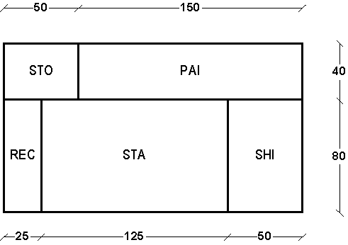
Figure 4.19. Block Layout for the Given Graph for the Autoparts Example
Table 4.11. Distance Matrix for the Autoparts Example
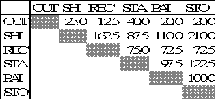
The distance matrix is then multiplied element by element with the symmetrical relationship matrix and the sum of the products is computed. This sum is the flow distance score and is equal to 49,525, of which 41,400 is between two departments and 8,125 is between departments and the outside.
Table 4.12. Penalty Shape Computations for the Autoparts Example

The total shape penalty is computed as the sum of the individual department shape penalties and is equal to 91,063. The total shape distance score for the layout is computed as the sum of the flow distance score and the shape penalty and is equal to 140,588.
The block layout without exchange improvements, the best block layout with the layered space allocation method, and the best block layout with the tiled space allocation method are shown in the next three figures. The distance statistics for the three layouts are shown in the next table.
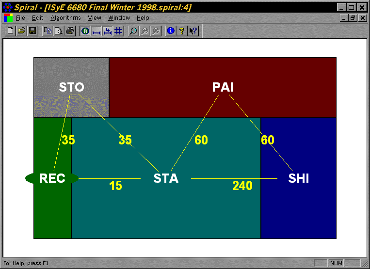
Figure 4.20. Unimproved Block Layout for the Given Graph for the Parts Example
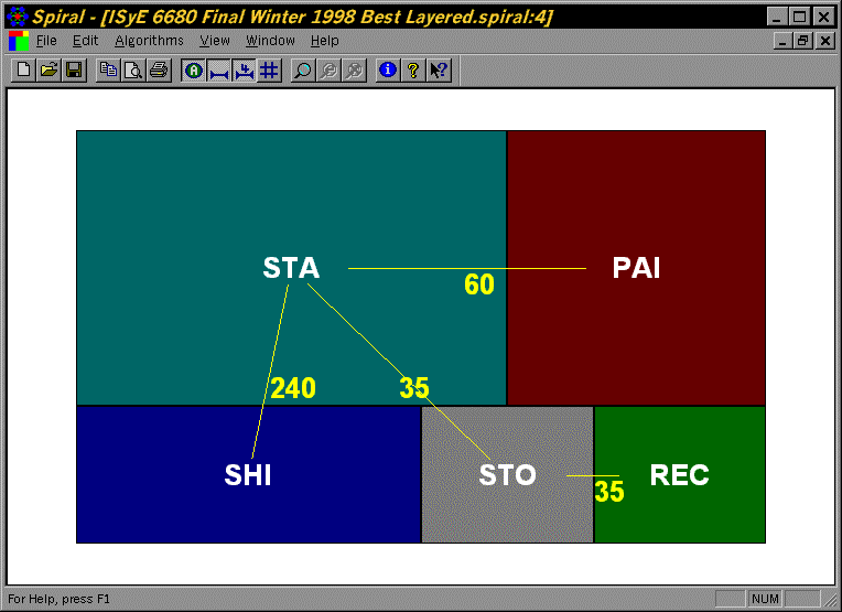
Figure 4.21. Best Layered Block Layout for the Given Graph for the Parts Example
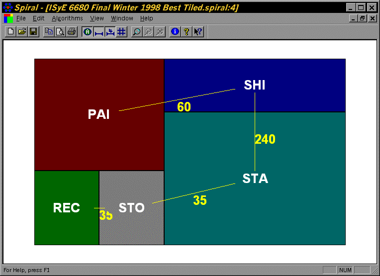
Figure 4.22. Best Tiled Block Layout for the Given Graph for the Parts Example
Table 4.13. Distance Statistics for the Parts Example

While the computer can provide evaluations of the different layouts based on centroid-to-centroid distances, it remains up to the user to decide which layout is best suited for their particular layout project.
